


We have much more to do and your continued support is needed now more than ever.
Smarter than Smart Meters: A New Approach to Building Energy Management
Imagine that you have just returned to the US after living for many years in a remote part of the world with little connection to the news of the day. As a lifelong baseball fan, you ask a friend, “How did our favorite baseball team the Houston Astros perform while I was away?” Your friend offers an unusual response: “In 2005 they scored 693 runs, and by 2007 their run production was up to 723 runs.” From the response you can conclude that their offense was more potent in 2007, but did the team actually improve?
The way most of us receive energy data at work and at home is in aggregated quantities such as kilowatt-hours and btus per month or per year. But like run totals in baseball, total energy units consumed is only a quantity, and drawing conclusions about the efficiency of a building just based on this quantity alone is as questionable as drawing conclusions solely on one team’s run production in baseball. After all, sometimes the data can deceive you. While the 2005 Astros only scored 693 runs, they went to the World Series. It was a season to remember. The 2007 Astros, despite plating 723 runs, finished in fourth place and both the manager and general manager were fired before Labor Day. It was a season to forget.
While literally millions of Americans — from die-hard fans to casual observers — understand the different measures to evaluate a baseball player and team (often in stunning detail), they have no such commensurate understanding for analyzing their utility bills. We simply have no feel for assessing the performance of conservation measures. We can sometimes answer the question “did we use more or less energy,” but not “did we use energy more or less efficiently?”
The first step, which many have taken, is to individually meter each building for each utility consumed (e.g. electricity, chilled water, steam). As the old management saying goes, you can’t manage what you don’t measure. But it’s also hard to manage what you measure inadequately. If we were to meter chilled water consumption for a campus building annually (i.e. the amount of cold water produced in a chiller at a campus utility plant and delivered in a pipe to that building over the course of a year to provide cooling), we might see totals such as 830,000 ton-hours in 2008, and 815,000 ton-hours in 2009. Other than to inform us about the total quantity of consumption (perhaps for billing purposes), the data is as potentially misleading as the annual run totals in the baseball example. We don’t know if in one year we operated the building more efficiently than the other. We don’t know how weather might have influenced consumption. We don’t know what times of the day, week, month, or year consumption might have been abnormally high or abnormally low (and we don’t know what abnormal is either). While monthly data provides clues about the seasonal variation in consumption, it is otherwise fraught with the same issues described above. Imagine, then, the challenge of justifying proposed capital investments in energy conservation projects, or evaluating the effectiveness of completed projects, when numbers on actual savings are misleading.
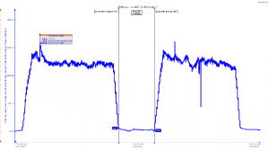
| Breaking out consumption by hour helps to pinpoint how efficient the system is under certain conditions. |
The next step is to provide near real time web-accessible meter readings that show exact consumption data at any given time during the day. Such data enables timely investigations to uncover potential problems, and greatly improves the effectiveness of troubleshooting. Consider Figure 1, which shows the actual consumption of chilled water for a two-day period in August 2009 for one of our campus buildings, Sewall Hall. The blue line shows the shape of chilled water consumption for the building over that time, which is considerably more useful than a single reading aggregating an entire day (or week, or month). We see quite clearly that the chilled water has a hard spike in the early morning, which would have remained undetected in a world of traditional meter readings. (If all campus buildings were to exhibit this start-up behavior, the Central Plant would be in disarray trying to react to it.) The consumption then settles in the range of about 120 tons of chilled water per hour across the daytime and into the evening.
We can also see that between 10 and 11PM chilled water consumption drops to almost zero, thanks to the implementation of a campus building temperature policy about one month prior to the days shown in Figure 1. Indoor temperature is allowed to drift upwards during the overnight hours, and then between 6 and 7AM the building is cooled back down just in time for the arrival of the first employees and the morning custodial team. This consumption profile makes sense for Sewall Hall, a building with classrooms, academic offices, and an art gallery, all of which are typically used only between the hours of 8AM to 10PM.
So, Figure 1 represents an example of the type of data that is displayed in today’s building energy dashboards and other smart meter applications. Recall, however, that we want to answer the question of whether we are using energy more or less efficiently, not whether we are using more or less in total. We want to get beyond run production, and start talking about wins and losses. While the data displayed in Figure 1 is certainly useful, and may even influence behavior when properly presented, one cannot make claims about verifiable energy savings based on this alone. Can someone claim that the savings from the nighttime setback should be calculated as roughly 125 tons of chilled water (if you extend the daytime consumption) across an approximately 8-hour time-span, or 1000 ton-hours of chilled water per night? Using a methodology and suite of tools developed by Rice University energy managers over the past decade and a half, you will see that the answer is no.
The energy consumption of a building from one time period to the next is influenced by a number of variables, including outdoor enthalpy (a combination of temperature and humidity), indoor enthalpy, time of day, day of the week, and day of the year. In Figure 1, the second day could have been significantly warmer or more humid than the first. Or perhaps heavy clouds rolled in from the Gulf of Mexico, reducing daytime peak temperatures. The first evening could have been exceptionally cool, or stifling and sticky. To properly account for these issues, our energy managers have created weather-normalized baseline models for chilled water, steam, and electrical consumption for many of our campus buildings. These baselines define the building’s operational personality, be it a well-behaved building or a building behaving poorly. These personalities are derived from how the building actually operates, regardless of the building’s design specifications. By then comparing these baselines against actual meter data, we can finally verify building energy savings.
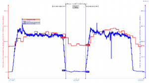
| The second figure shows how the baseline adjusts to account for changes in weather or usage. |
Figure 2 represents the next big step in building energy management. You will see the same consumption profile from the meter (in blue) that was shown in Figure 1. Displayed in red is a weather-normalized baseline model for chilled water consumption for Sewall Hall. This tells us how much chilled water we would expect to be consumed at Sewall Hall at any given time. Observe how the model changes during the day and night, and note that on day two the red line reaches a bit higher than on day one. This reflects higher enthalpy on day two, meaning we would expect to consume more chilled water to account for this particular weather condition versus day one. The weather guessing game has been removed — we don’t need to recall if one day was humid or the next was hot but unusually dry, because the baseline adjusts to account for it.
Now look specifically at the red and blue lines of Figure 2 as they relate to one another. The model provides the context for truly understanding consumption. We see that on both days, we are indeed wasting energy as the building starts up in the morning, as the blue line of actual consumption exceeds the red line of the predictive model. Then consumption of chilled water tends to track the model closely across the late morning, afternoon, and into the evening. What we see though once consumption drops sharply after 10PM is that the model – constructed from historical data of building energy consumption for a given enthalpy – reduces as well, but only down to about 90 tons of chilled water per hour, not zero. The nighttime setback is a new wrinkle. What the model shows is how chilled water consumption historically declined overnight as the final classes would let out and the last faculty and staff would go home, leaving an otherwise almost empty building to operate as if it were a 24-hour facility. Therefore, the savings in chilled water for the night of August 17-18th is not the 1,000 tons of chilled water as estimated above, but more like 90 tons of chilled water per hour across an 8-hour time period, or about 720 ton-hours of chilled water. This is 28% less than the initial estimate, and far more precise. If we assume a cost of chilled water of $0.16 per ton-hour, then we can report to our administrators with confidence that the savings in chilled water due to the nighttime setbacks in Sewall Hall for the night of August 17-18th, 2009 was about $115.20. That’s a win. And, by plotting the meter data against the model, we know that we are wasting energy due to the hard starts in the morning, and we can quantify exactly how much. Thanks to our new model, each morning at Rice doesn’t begin with a consumption profile that looks like a stalagmite.
The ability to plot meter data against a predictive baseline is a game-changer. At Rice, every two weeks we hold an interdepartmental committee meeting to review the performance of a number of our campus buildings using this tool. Participants represent maintenance, the central plant, housing and dining, project management and engineering, utility management, custodial, and sustainability. In addition, several members of this committee use these tools daily to assess performance, quantify savings, and identify problem areas. We can now accurately answer the question “did we use energy more or less efficiently?” – not just “did we use more or less?” – an answer that positions us to implement, understand, and verify the effect of energy conservation measures, to report real savings, and to quantify the resulting greenhouse gas emissions reductions from those conservation measures, all without wondering how weather may have affected the data.
The approach to energy management developed at Rice is now embedded in a campus energy management system that connects many disparate data sources, including several building controls systems, various district cooling plant systems, and the internet. We are creating dashboards for building lobbies, with weather-normalized energy and carbon reporting at the building-level. However, this approach needs to spread far beyond just campus environments. (So far, Rice, Dartmouth, the University of Iowa and the city of Houston are the only organizations I know that use this system.) A simple display of actual vs. expected energy consumption, in a manner easily understood by everyone from facility managers to employees to homeowners to tenants, is the next “killer app” of building energy technology. By putting the consumption data in context, what was once an abstract and confusing quantity for the average person is given meaning, much as comparing runs scored for one baseball team versus runs scored by their opponents gives the quantity meaning. Now we know how to tell whether and when we are truly using energy in buildings more efficiently or not. For energy management, the game has changed.
 Richard Johnson is the Director of Sustainability for Rice University. He also serves as the Associate Director of the Center for the Study of Environment and Society (CSES). Richard holds an appointment as a Professor in the Practice of Environmental Studies in Sociology and has taught several classes at Rice. Richard is also a research fellow for the Center on Race, Religion, and Urban Life (CORRUL). Richard received a B.S. in Civil Engineering from Rice University, and a Masters in Urban and Environmental Planning from the University of Virginia.
The author wishes to acknowledge the work of Mark Gardner and Eric Valentine, who have demonstrated that facilities departments can be a source of innovation and entrepreneurship, as well as John Windham, whose prowess in squeezing energy savings from campus buildings is now closely and accurately measured using Mark and Eric’s software.
